Friday, July 18, 2008

3d Surface Reconstruction

Recent project on 3d surface reconstruction based on calibrated camera and projector using the structured light technique.


Thursday, December 20, 2007

IBM T40 Internal Modem

The driver for the part of internal modem is loadable from snd_intel8x0m module. To create a modem device, download slmodemd which creates a node at /dev/ttySL0 for the modem which later can be used for the connection via PPP. Enable alsa mode (README) when installing slmodemd.
To run:
modprobe snd_intel8x0m
slmodemd --alsa hw:1

Saturday, November 24, 2007

Options delta hedging and volatility arbitrage

In options theory, delta is one of the greeks parameter that defines the sensitivity of the options price to the underlying asset price. Now, if we hold a portfolio consisting of 1 call option and delta number of corresponding stock (underlying asset), we have created a delta neutral portfolio. Theoretically, the price of portfolio is neutral to any small change of the stock price (note, delta is 1st order derivative) and will earn the risk free rate over a very short period of time. This is one of the reasoning that could be used to derive the famous Black-Scholes PDE. The reason that this applies to only small change in both price and time is because there are other parameters that affect the price of the option, namely gamma and theta.Now, gamma is defined as the measure of the rate of change in the delta (2nd order derivative) and theta is the measure of price sensitivity to the passage of time, thereby they explain the small change constraint.
Mathematically, for call option (european in particular), delta is defined as:

where c is the call option price, and S is the current stock price, N(d1) is the cdf of standard normal distribution defined within 0 and 1. The figure below will explain the delta concept.

The figure shows the call price with respect to the corresponding stock price. As we can see, the red line shows the slope of the curve at one particular stock price. This the delta of the call price at that particular stock price. Above that point, the call price increases at a greater rate than the stock price, and below that point the call price decreases at a slower rate. This is defined by the gamma parameter of the option, i.e. the rate of change of delta.
Now, here comes the interesting part, looking at the curve, one might wonder if there is an exploit such that under volatile market, profit could be earned irrespective of the direction of stock price with no initial investment at all (free lunch and/or arbitrage). Well, there is actually, I believe this is the so-called volatility arbitrage. This is done, again, by setting a portfolio consisting of long call and short delta number of stock price, as explained in the beginning.
Now, let's do some matlab simulations. The code for the simulation is given below:
function value = voltrade(S0,X,r,mu,t,sig,steps,NoPaths)
dt = t/steps;
drift = (mu - 0.5 * sig ^ 2) * dt;
vol = sig * sqrt(dt);
[price, delta, gamma] = tri_Eprice(S0, X, r, t, steps, sig, 0, 1);
Z = [zeros(NoPaths, 1) normrnd(drift, vol, NoPaths, steps)];
Z = (cumsum (Z'))';
S = S0*exp(Z);
ttm= [ones(NoPaths, steps) * dt];
ttm = cumsum (ttm')';
flipttm = [fliplr(ttm) (zeros(NoPaths, 1)+0.0000001)];
ttm = [(zeros(NoPaths, 1)+0.0000001) ttm];
callprice = blackscholes(S, X, r, flipttm, sig, 0) .* exp(-r.*ttm);
Sp = S .* exp(-r.*ttm);
value = mean(callprice - callprice(1,1) + (S0 - Sp) * delta);
subplot (2,1,1);
plot (value);
xlabel ('time step');
ylabel ('portfolio return');
subplot (2,1,2);
plot (mean(S));
xlabel ('time step');
ylabel ('stock price');
Note, the above function will call some external functions that are not defined here. Anyway, the objective of the function is to generate Monte Carlo simulation of stock prices, and at each time step to find the corresponding call option price, and also then to find the return of portfolio based on longing one call option and shorting delta number of stock. The function parameters are : S0 (current stock price), X (call option exercise price), r (risk free rate), mu (expected stock return), t (time to maturity), sig (volatility of stock), steps (number of delta t), and NoPaths (number of paths for Monte Carlo simulation).
Anyway, let's just run the function, first let's see what happen when the expected stock return, mu, is set to 30 % (which is set to be large enough to provide a greater certainty of large positive return, as the simulation doesn't really involve change in volatility parameter in order to explain the concept)
voltrade (50,50,0.05,0.3,0.5,0.4,1000,1000);
The return of the portfolio would look as below:

As you can see, the portfolio, will generate an "expected" positive return of approx. $ 0.8 after 6 months with zero initial investment. It is "expected" because, well, it's only a simulation based on Monte Carlo, which is then based on random numbers generated from certain distribution (lognormal) that is assumed to mimic certain parameters of stock price (there are a lot of assumptions here, this is finance, talking mostly about uncertainty).
Ok, now, let's see what happen if the stock generate an expected negative return (setting mu to -30%):
voltrade (50,50,0.05,-0.3,0.5,0.4,1000,1000);
The result:

As we can readily see, the expected portfolio return is positive even when the stock price declines within the period to maturity. Again, this is done with no initial investment at all (well, except the transaction costs).
Now, what if we set the expected stock return to 0:
voltrade (50,50,0.05,0.0,0.5,0.4,1000,1000);

Well, can't really see anything here but as the expected stock return follows a generalized Wiener process, there is always a probability of large change in price even though mu is set to zero. We could rerun the simulation over and over again and once in a while (lots of while, depends on volatility) the stock will change drastically, either up or down, and the option price will increase correspondingly (in real life, this is the right time to close the portfolio). This is more easily said than done in real life though (can't redo). Note, the simulation above doesn't really involve changes in volatility parameter. Hence, by incorporating an increase in volatility in between the time steps to maturity, the option price will generally increase, even though we set mu to zero. Hence, this strategy will perform well when the current implied volatility is low, and the investor expects that the volatility will increase considerably in the near future. The consideration for sensitivity of the option price with respect to volatility is set by the option greek parameter vega.

Update:
The above explanation and implementation are flawed, refer to here.

Sunday, November 18, 2007

Remote Desktop via Xming

Xming is a port of the X Window System to the Microsoft Windows operating system. Basically, it runs an X Server on your Windows machine, and client application can be run on the remote Linux machine (LM) and displayed on your Windows machine (WM).

To use it, you'll have to install Xming and putty on WM. Now run Xming X Server on localhost:0.0. Then, use Putty to connect to LM, and don't forget to enable X11 forwarding as shown below.


Most probably, X11 forwarding is not enabled on your LM ssh daemon. So change /etc/ssh/sshd_config to include:


X11Forwarding yes
X11DisplayOffset 10
X11UseLocalhost yes
And, restart sshd
/etc/rc.d/rc.sshd restart
Now, you'll need to re-ssh to LM using Putty. Check the event log ensure that "X11 forwarding enabled" is there and on the terminal type echo $DISPLAY whether it's been set by Putty.

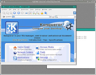
Well, that be it. I ran konqueror, and the result is as shown below.

Saturday, November 17, 2007

Remote Desktop to your home Linux PC via tightVNC

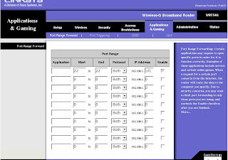
TightVNC is a free remote control software package derived from the popular VNC software. Download and install in the Linux PC here. It works in a client server manner where the server is the Linux home PC and the client is the PC from where you want to connect to the server to get the desktop of it. It's insecure as it doesn't contain any encryption apart from the initial user acknowledgment password. Hence, to make it secure we have to use use SSH tunneling. More info here and here. If the home server is firewalled or connected to the outside world via a router, don't forget to enable port forwarding.

In the snapshot above, all connection to port 22 on the router is forwarded to the IP address of the server.
To connect from the client PC, we have to connect to the external IP address of the router. Check your router IP here. The next step is to download putty and vncviewer client from here and here. These are the executables that you want to run from the client PC, and no installation is needed at all. Run Putty with tunneling, and forward client port e.g. 5901 to server port. Next, run the vncviewer client. Sample run would be like below:

Note: ssh tunneling makes the implementation rather slow, as it requires encryption and decryption, thereby bandwidth conservation is required. For example in the server I would run with the command : vncserver -geometry 800x600 depth 16 :01
and ~/.vnc/xstartup would look like below (it's the default actually, note the twm window manager is chosen):
xrdb $HOME/.Xresources
xsetroot -solid grey
xterm -geometry 80x24+10+10 -ls -title "$VNCDESKTOP Desktop" &
twm &

Sunday, November 11, 2007

Random number challenge

I read a blog post by Ariya Hidayat on a challenge to generate discrete integer random number 1..7 given a function that is able to generate random numbers (discrete integer) 1..5. This is my answer from the computer engineering point of view:

int r,x;
do{
do{
r = rand5();

if (r > 2 && r <= 4) x = rand5() + 5;

else if (r <= 2) x = rand5();

}while (r > 4);
}while (x > 7);
return x;

This answer is actually a bad one, at least compared to Ariya's answer in the sense that the probability that a call to this function will generate the respective random number directly without involving the loop is really low. Huh ?!?!? Okay, basically let me say that the inner loop will generate hit 80 % of the time. Why? Because there are 5 possibilities, and 4 of them are used to generate discrete integer random number 1..10 while 1 is deliberately ignored. Meanwhile, the outer loop will obviously generate 70 % hit. So, in the end the code will be effective 56 % (as in 80 % x 70 %, right ?) of the time without involving any loop. Actually, I think Ariya's answers are some of the most efficient implementations possible, especially the first one, hehe. Had I seen the challenge earlier, I wouldn't have been able to generate an implementation of the same quality, it would be so so like the above :(.
Now, let's take a glimpse from the mathematical point of view. If you've taken at least one math subject in your undergrad, I believe you should have heard of this term called central limit theorem. Huh?!? what's that?!? hehe, read here. I only know the basic. Basically, if you sum up m random numbers of the same property(mean, variance, etc) you'll end up with a random number with the property of normal distribution with mean m times the original mean and with variance m times the the original mean. So now, you have the ability to generate random number 1..5, and from this you're able to get some normally distributed random numbers, what's next? First, let's see the code to generate rand5 (implemented in matlab for laziness reason).

function r = rand5(m,n)
r = floor(5 * rand(m,n) + 1);
This code will generate a matrix of m row and n column of discrete random numbers. Let's see the code to generate rand7.

function r = rand7(n)
m = 1000;
sig = sqrt(2);
mu = 3;
temp = sum(rand5(m,n));
zn = (temp - m * mu)/(sig * sqrt(m));
x=0.5*erfc(-zn/sqrt(2));
r = floor(mod(x*70,7))+1;

The code above will generate a vector of n discrete random numbers 1..7.
So, how it works? The sig variable is obviously the standard deviation (sqrt of variance) of the random number generated by rand5, while mu is the mean of it which is 3 (correct? (1 + 2 + 3 + 4 + 5)/5 = ?). Now we call the rand5 to generate m by n matrix of it and sum it column by column, hence we get a vector of m number of rows and put it to variable temp. I put m to 1000 here(I know it s*cks and too large and not practical, but my purpose here is to learn something rite :p) such that it is large enough to generate a normal distribution with mean m * mu and standard deviation sig * sqrt(m). The next step is to convert it to standard normal distribution random number zn with mean 0 and standard deviation 1. Finally, convert it to uniform distribution by virtue of standard normal distribution cumulative distribution function(cdf). Again, another uncommon name. Well, basically in the program sense, cdf(x) gives the probabilty (from 0 to 1 obviously) that a random number generator will generate random number less or equal than x with some distribution (normal here) property. So here we get a uniform distribution which seems continous from 0 to 1 but actually it's discrete (and depends on m{that's why the larger the better, as I've told you}). The next step is trivial and obvious.
Now, by calling rand7 function so many times, we are able to generate so many random numbers that we could get a histogram of them. First, let's see the histogram of zn.


As we can see, it is indeed normally distributed with mean 0 (obvious) and variance 1 (unless you're a statistic professor you can't readily see it).
Now, let's check the histogram of rand7.

As we can, not so obviously, see, it is indeed uniformly distributed with discrete integer state 1..7. Cool huh !?! Well, that's about it.
Anyway, this method will make you look knowledgeable and yet at the same time stupid and dumb (because of redundancy and not much logic in it) in front of your interviewer and in the end it's not fun at all as you couldn't "tease" your interviewer with it and it's actually not "harmless" if you don't code in matlab as it requires some matrix and vector optimization to speed up your code in such large numbers of array manipulation.